Build Algorithm-Agnostic ML Pipelines in a Breeze

on the topic of algorithm-agnostic model building. You can find the previous two articles published on TDS below. 

Algorithm-Agnostic Model Building with MLflow

Explainable Generic ML Pipeline with MLflow

After writing these two articles, I continued to develop the framework, and it gradually evolved into something much larger than I originally envisioned. Rather than squeezing everything into another article, I decided to package it as an open-source Python library called MLarena to share with fellow data and ML practitioners. MLarena is an algorithm-agnostic machine learning toolkit that supports model training, diagnostics, and optimization.

🔗You can find the full codebase on GitHub: MLarena repo 🧰

At its core, MLarena is implemented as a custom mlflow.pyfunc model. This makes it fully compatible with the MLflow ecosystem, enabling robust experiment tracking, model versioning, and seamless deployment, regardless of which underlying ML library you use, and enables smooth migration between algorithms when necessary.

In addition, it also seeks to strike a balance between automation and expert insight in model development. Many tools either abstract away too much, making it hard to understand what’s happening under the hood, or require so much boilerplate that they slow down iteration. MLarena aims to bridge that gap: it automates routine machine learning tasks using best practices, while also providing tools for expert users to diagnose, interpret, and optimize their models more effectively.

In the sections that follow, we’ll look at how these ideas are reflected in the toolkit’s design and walk through practical examples of how it can support real-world machine learning workflows.

---

1. A Lightweight Abstraction for Training and Evaluation

One of the recurring pain points in ML workflows is the amount of boilerplate code required just to get a working pipeline, especially when switching between algorithms or frameworks. MLarena introduces a lightweight abstraction that standardizes this process while remaining compatible with scikit-learn-style estimators. 

Here’s a simple example of how the core MLPipeline object works:

from mlarena import MLPipeline, PreProcessor

# Define the pipeline
mlpipeline_rf = MLPipeline(
    model = RandomForestClassifier(), # works with any sklearn style algorithm
    preprocessor = PreProcessor() 
)
# Fit the pipeline
mlpipeline_rf.fit(X_train,y_train)
# Predict on new data and evaluate
results = mlpipeline_rf.evaluate(X_test, y_test)

This interface wraps together common preprocessing steps, model training, and evaluation. Internally, it auto-detects the task type (classification or regression), applies appropriate metrics, and generates a diagnostic report—all without sacrificing flexibility in how models or preprocessors are defined (more on customization options later).

Rather than abstracting everything away, MLarena focuses on surfacing meaningful defaults and insights. The evaluate method doesn’t just return scores, it produces a full report tailored to the task.

1.1 Diagnostic Reporting

For classification tasks, the evaluation report includes key metrics such as AUC, MCC, precision, recall, F1, and F-beta (when beta is specified). The visual outputs feature a ROC-AUC curve (bottom left), a confusion matrix (bottom right), and a precision–recall–threshold plot at the top. In this top plot, precision (blue), recall (red), and F-beta (green, with β = 1 by default) are shown across different classification thresholds, with a vertical dotted line indicating the current threshold to highlight the trade-off. These visualizations are useful not only for technical diagnostics, but also for supporting discussions around threshold selection with domain experts (more on threshold optimization later).

=== Classification Model Evaluation ===

1. Evaluation Parameters
----------------------------------------
• Threshold:   0.500    (Classification cutoff)
• Beta:        1.000    (F-beta weight parameter)

2. Core Performance Metrics
----------------------------------------
• Accuracy:    0.805    (Overall correct predictions)
• AUC:         0.876    (Ranking quality)
• Log Loss:    0.464    (Confidence-weighted error)
• Precision:   0.838    (True positives / Predicted positives)
• Recall:      0.703    (True positives / Actual positives)
• F1 Score:    0.765    (Harmonic mean of Precision & Recall)
• MCC:         0.608    (Matthews Correlation Coefficient)

3. Prediction Distribution
----------------------------------------
• Pos Rate:    0.378    (Fraction of positive predictions)
• Base Rate:   0.450    (Actual positive class rate)

For regression models, MLarena automatically adapts its evaluation metrics and visualisations:

=== Regression Model Evaluation ===

1. Error Metrics
----------------------------------------
• RMSE:         0.460      (Root Mean Squared Error)
• MAE:          0.305      (Mean Absolute Error)
• Median AE:    0.200      (Median Absolute Error)
• NRMSE Mean:   22.4%      (RMSE/mean)
• NRMSE Std:    40.2%      (RMSE/std)
• NRMSE IQR:    32.0%      (RMSE/IQR)
• MAPE:         17.7%      (Mean Abs % Error, excl. zeros)
• SMAPE:        15.9%      (Symmetric Mean Abs % Error)

2. Goodness of Fit
----------------------------------------
• R²:           0.839      (Coefficient of Determination)
• Adj. R²:      0.838      (Adjusted for # of features)

3. Improvement over Baseline
----------------------------------------
• vs Mean:      59.8%      (RMSE improvement)
• vs Median:    60.9%      (RMSE improvement)

One danger in rapid iteration of ML project is that some underlying issues may go unnoticed. Therefore, in addition to the above metrics and plots, a Model Evaluation Diagnostics section will appear in the report when potential red flags are detected:

Regression Diagnostics

⚠️ Sample-to-feature ratio warnings: Alerts when n/k < 10, indicating high overfitting risk
ℹ️ MAPE transparency: Reports how many observations were excluded from MAPE due to zero target values

Classification Diagnostics

⚠️ Data leakage detection: Flags near-perfect AUC (>99%) that often indicates leakage
⚠️ Overfitting alerts: Same n/k ratio warnings as regression
ℹ️ Class imbalance awareness: Flags severely imbalanced class distributions

Below is an overview of MLarena’s evaluation reports for both classification and regression tasks:

1.2 Explainability as a Built-In Layer

Explainability in machine learning projects is crucial for multiple reasons:

1. Model Selection
   Explainability helps us choose the best model by letting us evaluate the soundness of its reasoning. Even if two models show similar performance metrics, examining the features they rely on with domain experts can reveal which model’s logic aligns better with real-world understanding.
2. Troubleshooting
   Analyzing a model’s reasoning is a powerful troubleshooting strategy for improvement. For instance, by investigating why a classification model confidently made a mistake, we can pinpoint the contributing features and correct its reasoning.
3. Model Monitoring
   Beyond typical performance and data drift checks, monitoring model reasoning is highly informative. Getting alerted to significant shifts in the key features driving a production model’s decisions helps maintain its reliability and relevance.
4. Model Implementation
   Providing model reasoning alongside predictions can be incredibly valuable to end-users. For example, a customer service agent could use a churn score along with the specific customer features that lead to that score to better retain a customer.

To support model interpretability, the explain_model method gives you global explanations, revealing which features have the most significant impact on your model’s predictions.

mlpipeline.explain_model(X_test)

The explain_case method provides local explanations for individual cases, helping us understand how each feature contributes to each specific prediction.

mlpipeline.explain_case(5)

1.3 Reproducibility and Deployment Without Extra Overhead

One persistent challenge in machine learning projects is ensuring that models are reproducible and production-ready—not just as code, but as complete artifacts that include preprocessing, model logic, and metadata. Often, the path from a working notebook to a deployable model involves manually wiring together multiple components and remembering to track all relevant configurations.

To reduce this friction, MLPipeline is implemented as a custom mlflow.pyfunc model. This design choice allows the entire pipeline ( including the preprocessing steps and trained model), to be packaged as a single, portable artifact.

When evaluating a pipeline, you can enable MLflow logging by setting log_model=True:

results = mlpipeline.evaluate(
    X_test, y_test, 
    log_model=True # to log the pipeline with mlflow
)

Behind the scenes, this triggers a series of MLflow operations:

• Starts and manages an MLflow run
• Logs model hyperparameters and evaluation metrics
• Saves the complete pipeline object as a versioned artifact
• Automatically infers the model signature to reduce deployment errors

This helps teams maintain experiment traceability and move from experimentation to deployment more smoothly, without duplicating tracking or serialization code. The resulting artifact is compatible with the MLflow Model Registry and can be deployed through any of MLflow’s supported backends.

2. Tuning Models with Efficiency and Stability in Mind

Hyperparameter tuning is one of the most resource-intensive parts of building machine learning models. While search techniques like grid or random search are common, they can be computationally expensive and often inefficient, especially when applied to large or complex search spaces. Another big concern in hyperparameter optimization is that it could produce unstable models that perform well in development but degrade in production.

To address these issues, MLarena includes a tune method that simplifies the process of hyperparameter optimization while encouraging robustness and transparency. It builds on Bayesian optimization—an efficient search strategy that adapts based on previous results—and adds guardrails to avoid common pitfalls like overfitting or incomplete search space coverage.

2.1 Hyperparameter Optimization with Built-In Early Stopping and Variance Control

Here’s an example of how to run tuning using LightGBM and a custom search space:

from mlarena import MLPipeline, PreProcessor
import lightgbm as lgb

lgb_param_ranges = {
    'learning_rate': (0.01, 0.1),  
    'n_estimators': (100, 1000),   
    'num_leaves': (20, 100),
    'max_depth': (5, 15),
    'colsample_bytree': (0.6, 1.0),
    'subsample': (0.6, 0.9)
}

# setting up with default settings, see customization below 
best_pipeline = MLPipeline.tune(
    X_train, 
    y_train,
    algorithm=lgb.LGBMClassifier, # works with any sklearn style algorithm
    preprocessor=PreProcessor(),
    param_ranges=lgb_param_ranges 
    )

To avoid unnecessary computation, the tuning process includes support for early stopping: you can set a maximum number of evaluations, and stop the process automatically if no improvement is observed after a specified number of trials. This saves computation time while focusing the search on the most promising parts of the search space.

best_pipeline = MLPipeline.tune(
    ... 
    max_evals=500,       # maximum optimization iterations
    early_stopping=50,   # stop if no improvement after 50 trials
    n_startup_trials=5,  # minimum trials before early stopping kicks in
    n_warmup_steps=0,    # steps per trial before pruning    
    )

To ensure robust results, MLarena applies cross-validation during hyperparameter tuning. Beyond optimizing for average performance, it also allows you to penalize high variance across folds using the cv_variance_penalty parameter. This is particularly valuable in real-world scenarios where model stability can be just as important as raw accuracy.

best_pipeline = MLPipeline.tune(
    ...
    cv=5,                    # number of folds for cross-validation
    cv_variance_penalty=0.3, # penalize high variance across folds
    )

For example, between two models with identical mean AUC, the one with lower variance across folds is often more reliable in production. It will be selected by MLarena tuning due to its better effective score, which is mean_auc - std * cv_variance_penalty:

Model	Mean AUC	Std Dev	Effective Score
A	0.85	0.02	0.85 – 0.02 * 0.3 (penalty)
B	0.85	0.10	0.85 – 0.10 * 0.3 (penalty)

2.2 Diagnosing Search Space Design with Visual Feedback

Another frequent bottleneck in tuning is designing a good search space. If the range for a hyperparameter is too narrow or too broad, the optimizer may waste iterations or miss high-performing regions entirely.

To support more informed search design, MLarena includes a parallel coordinates plot that visualizes how different hyperparameter values relate to model performance:

• You can spot trends, such as which ranges of learning_rate consistently yield better results.
• You can identify edge clustering, where top-performing trials are bunched at the boundary of a parameter range, often a sign that the range needs adjustment.
• You can see interactions across multiple hyperparameters, helping refine your intuition or guide further exploration.

This kind of visualization helps users refine search spaces iteratively, leading to better results with fewer iterations.

best_pipeline = MLPipeline.tune(
    ...
    # to show parallel coordinate plot:
    visualize = True # default=True
    )

2.3 Choosing the Right Metric for the Problem

The objective of tuning isn’t always the same: in some cases, you want to maximize AUC, in others, you may care more about minimizing RMSE or SMAPE. But different metrics also require different optimization directions—and when combined with cross-validation variance penalty, which either needs to be added to or subtracted from the CV mean depending on the optimization direction, the math can get tedious. 😅

MLarena simplifies this by supporting a wide range of metrics for both classification and regression:

Classification metrics:

• auc (default)
• f1
• accuracy
• log_loss
• mcc

Regression metrics:

• rmse (default)
• mae
• median_ae
• smape
• nrmse_mean, nrmse_iqr, nrmse_std

To switch metrics, simply pass tune_metric to the method:

best_pipeline = MLPipeline.tune(
    ...
    tune_metric = "f1"
    )

MLarena handles the rest, automatically determining whether the metric should be maximized or minimized and applying the variance penalty consistently.

3. Tackling Real-World Preprocessing Challenges

Preprocessing is often one of the most overlooked steps in machine learning workflows, and also one of the most error-prone. Dealing with missing values, high-cardinality categoricals, irrelevant features, and inconsistent column naming can introduce subtle bugs, degrade model performance, or block production deployment altogether.

MLarena’s PreProcessor was designed to make this step more robust and less ad hoc. It offers sensible defaults for common use cases, while providing the flexibility and tooling needed for more complex scenarios.

Here’s an example of the default configuration:

from mlarena import PreProcessor

preprocessor = PreProcessor(
    num_impute_strategy="median",          # Numeric missing value imputation
    cat_impute_strategy="most_frequent",   # Categorical missing value imputation
    target_encode_cols=None,               # Columns for target encoding (optional)
    target_encode_smooth="auto",           # Smoothing for target encoding
    drop="if_binary",                      # Drop strategy for one-hot encoding
    sanitize_feature_names=True            # Clean up special characters in column names
)

X_train_prep = preprocessor.fit_transform(X_train)
X_test_prep = preprocessor.transform(X_test)

These defaults are often sufficient for quick iteration. But real-world datasets rarely fit neatly into defaults. So let’s explore some of the more nuanced preprocessing tasks the PreProcessor supports.

3.1 Managing High-Cardinality Categoricals with Target Encoding

High-cardinality categorical features pose a challenge: traditional one-hot encoding can result in hundreds of sparse columns. Target encoding offers a compact alternative, replacing categories with smoothed averages of the target variable. However, tuning the smoothing parameter is tricky: too little smoothing leads to overfitting, while too much dilutes useful signal.

MLarena adopts the empirical Bayes-based approach in SKLearn’s TargetEncoder to smoothing when target_encode_smooth="auto", and also allows users to specify numeric values (see doc for sklearn TargetEncoder and Micci-Barrec, 2001).

preprocessor = PreProcessor(
    target_encode_cols=['city'],
    target_encode_smooth='auto'
)

To help guide this choice, the plot_target_encoding_comparison method visualizes how different smoothing values affect the encoding of rare categories. For example:

PreProcessor.plot_target_encoding_comparison(
    X_train, y_train,
    target_encode_col='city',
    smooth_params=['auto', 10, 20]
)

This is especially useful for inspecting the effect on underrepresented categories (e.g., a city like “Seattle” with only 24 samples). The visualization shows that different smoothing parameters lead to marked differences in Seattle’s encoded value. Such clear visuals support data specialists and domain experts in having meaningful discussions and making informed decisions on the best encoding strategy.

3.2 Identifying and Removing Unhelpful Features

Another common challenge is feature overload: too many variables, not all of which contribute meaningful signals. Selecting a cleaner subset can improve both performance and interpretability.

The filter_feature_selection method helps filter out:

• Features with high missingness
• Features with only one unique value
• Features with low mutual information with the target

Here’s how it works:

filter_fs = PreProcessor.filter_feature_selection(
    X_train,
    y_train,
    task='classification', # or 'regression'
    missing_threshold=0.2, # drop features with > 20% missing values
    mi_threshold=0.05,     # drop features with low mutual information
)

This returns a summary like:

Filter Feature Selection Summary:
==========
Total features analyzed: 7

1. High missing ratio (>20.0%): 0 columns

2. Single value: 1 columns
   Columns: occupation

3. Low mutual information (<0.05): 3 columns
   Columns: age, tenure, occupation

Recommended drops: (3 columns in total)

The selected features can be accessed programmatically:

selected_cols = fitler_fs['selected_cols']
X_train_selected = X_train[selected_cols]

This early filter step doesn’t replace full feature engineering or wrapper-based selection (which is on the roadmap), but helps reduce noise before heavier modelling begins.

3.3 Preventing Downstream Errors with Column Name Sanitization 

When one-hot encoding is applied to categorical features, column names can inherit special characters, like 'age_60+' or 'income_<$30K'. These characters can break pipelines downstream, especially during logging, deployment, or use with MLflow.

To reduce the risk of silent pipeline failures, MLarena automatically sanitizes feature names by default:

preprocessor = PreProcessor(sanitize_feature_names=True)

Characters like +, <, and % are replaced with safe alternatives as shown in the table below, improving compatibility with production-grade tooling. Users who prefer raw names can easily disable this behavior by setting sanitize_feature_names=False.

4. Solving Everyday Challenges in ML Practice

In real-world machine learning projects, success goes beyond model accuracy. It often depends on how clearly we communicate results, how well our tools support stakeholder decision-making, and how reliably our pipelines handle imperfect data. MLarena includes a growing set of utilities designed to address these practical challenges. Below are just a few examples.

4.1 Threshold Analysis for Classification Problems

Binary classification models often output probabilities, but real-world decisions require a hard threshold to separate positives from negatives. This choice affects precision, recall, and ultimately, business outcomes. Yet in practice, thresholds are often left at the default 0.5, even when that’s not aligned with domain needs.

MLarena’s threshold_analysis method helps make this choice more rigorous and tailored. We can:

• Customize the precision-recall balance via the beta parameter in the F-beta score
  

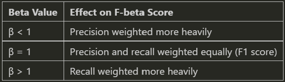
• Find the optimal classification threshold based on our business goals by maximizing F-beta
• Use bootstrapping or stratified k-fold cross-validation for robust, reliable estimates

# Perform threshold analysis using bootstrap method
results = MLPipeline.threshold_analysis(  
    y_train,                     # True labels for training data
    y_pred_proba,                # Predicted probabilities from model
    beta = 0.8,                  # F-beta score parameter (weights precision more than recall)
    method = "bootstrap",        # Use bootstrap resampling for robust results
    bootstrap_iterations=100)    # Number of bootstrap samples to generate

# utilize the optimal threshold identified on new data
best_pipeline.evaluate(
    X_test, y_test, beta=0.8, 
    threshold=results['optimal_threshold']
    )

This enables practitioners to tie model decisions more closely to domain priorities, such as catching more fraud cases (recall) or reducing false alarms in quality control (precision).

4.2 Communicating with Clarity Through Visualization

Strong visualizations are essential not just for EDA, but for engaging stakeholders and validating findings. MLarena includes a set of plotting utilities designed for interpretability and clarity.

4.2.1 Comparing Distributions Across Groups

When analyzing numerical data across distinct categories such as regions, cohorts, or treatment groups, a comprehensive understanding requires more than just central tendency metrics like mean or median. It’s crucial to also grasp the data’s dispersion and identify any outliers. To address this, the plot_box_scatter function in Mlarena overlays boxplots with jittered scatter points, providing rich distribution information within a single, intuitive visualization.

Furthermore, complementing visual insights with robust statistical analysis often proves invaluable. Therefore, the plotting function optionally integrates statistical tests such as ANOVA, Welch’s ANOVA, and Kruskal-Wallis, allowing us to annotate our plots with statistical test results, as demonstrated below. 

import mlarena.utils.plot_utils as put

fig, ax, results = put.plot_box_scatter(
    data=df,
    x="item",
    y="value",
    title="Boxplot with Scatter Overlay (Demo for Crowded Data)",
    point_size=2,
    xlabel=" "，
    stat_test="anova",      # specify a statistical test
    show_stat_test=True
    )

There are many ways to customize the plot — either by modifying the returned ax object or using built-in function parameters. For example, you can color the points by another variable using the point_hue parameter.

fig, ax = put.plot_box_scatter(
    data=df,
    x="group",
    y="value",
    point_hue="source", # color points by source
    point_alpha=0.5,
    title="Boxplot with Scatter Overlay (Demo for Point Hue)",
)

4.2.2 Visualizing Temporal Distribution

Data specialists and domain experts frequently need to observe how the distribution of a continuous variable evolves over time to spot critical shifts, emerging trends, or anomalies.

This often involves boilerplate tasks like aggregating data by desired time granularity (hourly, weekly, monthly, etc.), ensuring correct chronological order, and customizing appearances, such as coloring points by a third variable of interest. Our plot_distribution_over_time function handles these complexities with ease.

# automatically group data and format X-axis lable by specified granularity
fig, ax = put.plot_distribution_over_time(
    data=df,
    x='timestamp',
    y='heart_rate',
    freq='h',                                   # specify granularity
    point_hue=None,                             # set a variable to color points if desired
    title='Heart Rate Distribution Over Time',
    xlabel=' ',
    ylabel='Heart Rate (bpm)',
)

More demos of plotting functions and examples are available in the plot_utils documentation🔗. 

4.3 Data Utilities

If you’re like me, you probably spend a lot of time cleaning and troubleshooting data before getting to the fun parts of machine learning. 😅 Real-world data is often messy, inconsistent, and full of surprises. That’s why MLarena includes a growing collection of data_utils functions to simplify and streamline our EDA and data preparation process.

4.3.1 Cleaning Up Inconsistent Date Formats

Date columns don’t always arrive in clean, ISO formats, and inconsistent casing or formats can be a real headache. The transform_date_cols function helps standardize date columns for downstream analysis, even when values have irregular formats like:

import mlarena.utils.data_utils as dut

df_raw = pd.DataFrame({
    ...
    "date": ["25Aug2024", "15OCT2024", "01Dec2024"],  # inconsistent casing
})

# transformed the specified date columns
df_transformed = dut.transform_date_cols(df_raw, 'date', "%d%b%Y")
df_transformed['date']
# 0   2024-08-25
# 1   2024-10-15
# 2   2024-12-01

It automatically handles case variations and converts the column into proper datetime objects.

If you sometimes forget the Python date format codes or mix them up with Spark’s, you’re not alone 😁. Just check the function’s docstring for a quick refresher.

?dut.transform_date_cols  # check for docstring

Signature:
----------
dut.transform_date_cols(
    data: pandas.core.frame.DataFrame,
    date_cols: Union[str, List[str]],
    str_date_format: str = '%Y%m%d',
) -> pandas.core.frame.DataFrame
Docstring:
Transforms specified columns in a Pandas DataFrame to datetime format.

Parameters
----------
data : pd.DataFrame
    The input DataFrame.
date_cols : Union[str, List[str]]
    A column name or list of column names to be transformed to dates.
str_date_format : str, default="%Y%m%d"
    The string format of the dates, using Python's `strftime`/`strptime` directives.
    Common directives include:
        %d: Day of the month as a zero-padded decimal (e.g., 25)
        %m: Month as a zero-padded decimal number (e.g., 08)
        %b: Abbreviated month name (e.g., Aug)
        %B: Full month name (e.g., August)
        %Y: Four-digit year (e.g., 2024)
        %y: Two-digit year (e.g., 24)

4.3.2 Verifying Primary Keys in Messy Data

Identifying a valid primary key can be challenging in real-world, messy datasets. While a traditional primary key must inherently be unique across all rows and contain no missing values, potential key columns often contain nulls, particularly in the early stages of a data pipeline.

The is_primary_key function adopts a pragmatic approach to this challenge: it alerts user to any missing values within potential key columns and then verifies if the remaining non-null rows are uniquely identifiable.

This is useful for:

– Data quality assessment: Quickly assess the completeness and uniqueness of our key fields.
– Join readiness: Identify reliable keys for merging datasets, even when some values are initially missing.
– ETL validation: Verify key constraints while accounting for real-world data imperfections.
– Schema design: Inform robust database schema planning with insights derived from actual data key characteristics.

As such, is_primary_key is particularly valuable for designing resilient data pipelines in less-than-perfect data environments. It supports both single and composite keys by accepting either a column name or a list of columns.

df = pd.DataFrame({
    # Single column primary key
    'id': [1, 2, 3, 4, 5],    
    # Column with duplicates
    'category': ['A', 'B', 'A', 'B', 'C'],    
    # Date column with some duplicates
    'date': ['2024-01-01', '2024-01-01', '2024-01-02', '2024-01-02', '2024-01-03'],
    # Column with null values
    'code': ['X1', None, 'X3', 'X4', 'X5'],    
    # Values column
    'value': [100, 200, 300, 400, 500]
})

print("\nTest 1: Column with duplicates")
dut.is_primary_key(df, ['category'])  # Should return False

print("\nTest 2: Column with null values")
dut.is_primary_key(df, ['code','date']) # Should return True

Test 1: Column with duplicates
✅ There are no missing values in column 'category'.
ℹ️ Total row count after filtering out missings: 5
ℹ️ Unique row count after filtering out missings: 3
❌ The column(s) 'category' do not form a primary key.

Test 2: Column with null values
⚠️ There are 1 row(s) with missing values in column 'code'.
✅ There are no missing values in column 'date'.
ℹ️ Total row count after filtering out missings: 4
ℹ️ Unique row count after filtering out missings: 4
🔑 The column(s) 'code', 'date' form a primary key after removing rows with missing values.

---

Beyond what we’ve covered, the data_utils module offers other handy utilities, including a dedicated set of three functions for the “Discover → Investigate → Resolve” deduplication workflow, where is_primary_key discussed above, serves as the initial step. More details are available in the data_utils demo🔗. 

---

And there you have it — an introduction to the MLarena package. My hope is that these tools prove as valuable for streamlining your machine learning workflows as they have been for mine. This is an open-source, not-for-profit initiative. Please don’t hesitate to reach out if you have any questions or would like to request new features. I’d love to hear from you! 🤗

Stay tuned, and follow me on Medium. 😁

💼LinkedIn | 😺GitHub | 🕊️Twitter/X

---

Unless otherwise noted, all images are by the author.